model.diffusion
- class diffusion.model.DenoiseDiffusion(eps_model, n_steps)
Denoising diffusion probabilistic models introduced in Ho et al. [HJA20].
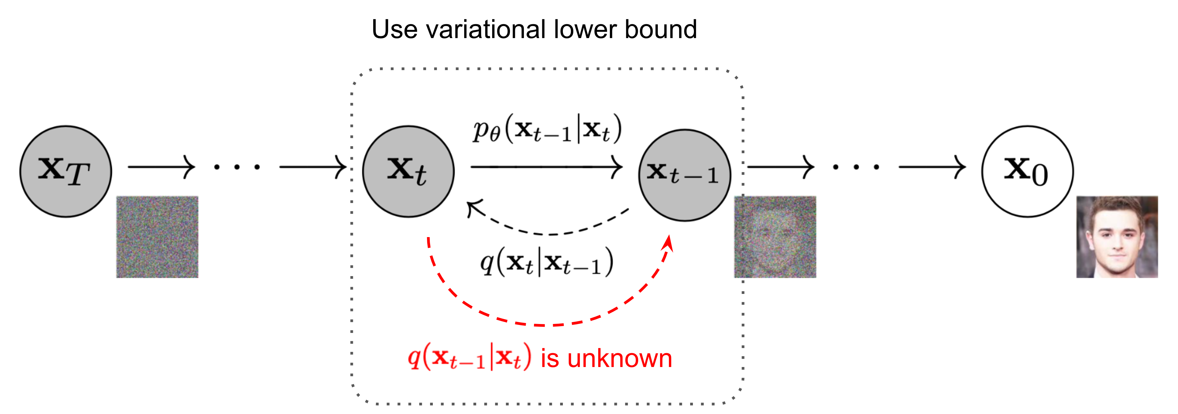
The Markov chain of forward (reverse) diffusion process of generating a sample by slowly adding (removing) noise. (Image source: Ho et al. [HJA20] with a few additional annotations)
See also
What are Diffusion Models? - Lilian Weng
Generative Modeling by Estimating Gradients of the Data Distribution - Yang Song
Forward Process
The forward diffusion process adds small amount of Gaussian noise to the data sampled from a real data distribution \(x_{0} \sim q\left(x_{0}\right)\) for \(T\) timesteps:
\[\begin{split}\begin{aligned} q\left(x_{1: T} \mid x_{0}\right) &=\prod_{t=1}^{T} q\left(x_{t} \mid x_{t-1}\right) \\ q\left(x_{t} \mid x_{t-1}\right) &=\mathcal{N}\left(x_{t} ; \sqrt{1-\beta_{t}} x_{t-1}, \beta_{t} \mathbf{I}\right) \end{aligned}\end{split}\]where \(\beta_{1}, \ldots, \beta_{T}\) is the variance schedule. (see
schedulemodule)Use reparameterization trick, then we can sample \(x_{t}\) at any timestep \(t\) with:
\[q\left(x_{t} \mid x_{0}\right) =\mathcal{N}\left(x_{t} ; \sqrt{\bar{\alpha}_{t}} x_{0}, \left(1-\bar{\alpha}_{t}\right) \mathbf{I}\right)\]where \(\alpha_{t}=1-\beta_{t}\) and \(\bar{\alpha}_{t}=\prod_{s=1}^{t} \alpha_{s}\).
See
q_sample()for more details.Reverse Process
The reverse diffusion process removes noise starting at \(p\left(x_{T}\right)=\mathcal{N}\left(x_{T} ; \mathbf{0}, \mathbf{I}\right)\) for \(T\) time steps (note that \(p\left(x_{0} \mid x_{t}\right)\) can not be calculated at any timestep \(t\) in one step):
\[\begin{split}\begin{aligned} p_{\theta}\left(x_{0: T}\right) &=p_{\theta}\left(x_{T}\right) \prod_{t=1}^{T} p_{\theta}\left(x_{t-1} \mid x_{t}\right) \\ p_{\theta}\left(x_{t-1} \mid x_{t}\right) &=\mathcal{N}\left(x_{t-1} ; \mu_{\theta}\left( x_{t}, t\right), \Sigma_{\theta}\left(x_{t}, t\right) \right) \end{aligned}\end{split}\]where \(\theta\) are the parameters we train.
See
p_sample()for more details.Loss function
Calculate simplifiled MSE (l2) loss:
\[L_{simple}(\theta)=\mathbb{E}_{t, x_{0}, \epsilon} \left[\left\|\epsilon-\epsilon_{\theta}\left(\sqrt{\bar{\alpha}_{t}} x_{0} +\sqrt{1-\bar{\alpha}_{t}} \epsilon, t\right)\right\|^{2}\right]\]See
loss()for more details.- Variables
eps_model – the \(\epsilon_{\theta}\left(x_{t}, t\right)\) denoise model.
n_steps – the number of timesteps \(T\).
beta – the \(\beta_{1}, \ldots, \beta_{T}\) generated from variance schedule. Once
betais given, the following notation’s value (eg.alpha) can be calculated during initialization, which is convenient for later process.alpha – it is defined that \(\alpha_{t}=1-\beta_{t}\).
alpha_bar – it is defined that \(\bar{\alpha}_{t}=\prod_{s=1}^{t} \alpha_{s}\).
sigma2 – The square of the standard deviation \(\sigma_{t}^{2}\), i.e the variance \(\Sigma_{t}\). In the forward process we simply assume that \(\sigma_{t}^{2} = \beta_{t} \mathbf{I}\).
- Parameters
- loss(x_0, noise=None)
Calculate simplifiled MSE (l2) loss:
\[L_{simple}(\theta)=\mathbb{E}_{t, x_{0}, \epsilon} \left[\left\|\epsilon-\epsilon_{\theta}\left(\sqrt{\bar{\alpha}_{t}} x_{0} +\sqrt{1-\bar{\alpha}_{t}} \epsilon, t\right)\right\|^{2}\right]\]where \(\epsilon_{\theta}\) is from the given \(\epsilon_{\theta}\left(x_{t}, t\right)\) model and \(x_{t}\) is from
q_sample().See the original paper for derivation details.
- p_sample(x_t, t)
Sample during the reverse diffusion process:
\[ \begin{align}\begin{aligned}p_{\theta}\left(x_{t-1} \mid x_{t}\right) =\mathcal{N}\left(x_{t-1} ; \mu_{\theta}\left(x_{t}, t\right), \sigma_{t}^{2} \mathbf{I}\right)\\\mu_{\theta}\left(x_{t}, t\right) =\frac{1}{\sqrt{\alpha_{t}}}\left(x_{t}-\frac{\beta_{t}}{\sqrt{1-\bar{\alpha}_{t}}} \epsilon_{\theta}\left(x_{t}, t\right)\right)\end{aligned}\end{align} \]
- q_sample(x_0, t, noise=None)
Sample during the the forward diffusion process:
\[q\left(x_{t} \mid x_{0}\right) =\mathcal{N}\left(x_{t} ; \sqrt{\bar{\alpha}_{t}} x_{0}, \left(1-\bar{\alpha}_{t}\right) \mathbf{I}\right)\]